CRSP Treasury Data Overview

The CRSP US Treasury Database is a comprehensive source of historical Treasury security data maintained by the Center for Research in Security Prices at the University of Chicago’s Booth School of Business. This section provides an essential overview of this critical dataset, which will serve as the foundation for our subsequent replication of the Gürkaynak, Sack, and Wright (2006) & Waggoner (1997) yield curve estimation methodologies.

Database Description

The CRSP US Treasury Database provides complete historical descriptive information and market data for US Treasury securities, including:

• Prices

• Returns

• Accrued interest

• Yields

• Durations

The database begins in 1961 and is updated monthly. The data is available in ASCII, Excel, and SAS formats.

import numpy as np
import pandas as pd
import matplotlib.pyplot as plt
from pathlib import Path

ROOT = Path.cwd()
PROJECT_ROOT = ROOT if (ROOT / 'src').exists() else ROOT.parent
DATA_DIR = PROJECT_ROOT / '_data'
OUTPUT_DIR = PROJECT_ROOT / '_output'

TREASURY_FILES = [
    'TFZ_consolidated.parquet',
    'TFZ_DAILY.parquet',
    'TFZ_INFO.parquet',
    'TFZ_with_runness.parquet'
]

for file in TREASURY_FILES:
    df = pd.read_parquet(DATA_DIR / file)
    print(f'Columns in {file}: {df.columns.tolist()}')

Columns in TFZ_consolidated.parquet: ['kytreasno', 'kycrspid', 'tcusip', 'mcaldt', 'tdatdt', 'tmatdt', 'tfcaldt', 'tfcpdt', 'tmbid', 'tmask', 'tmaccint', 'tmyld', 'price', 'tcouprt', 'itype', 'original_maturity', 'iflwr', 'years_to_maturity', 'tmduratn', 'tmretnua', 'days_to_maturity', 'callable']
Columns in TFZ_DAILY.parquet: ['kytreasno', 'kycrspid', 'mcaldt', 'tmbid', 'tmask', 'tmaccint', 'tmyld', 'price']
Columns in TFZ_INFO.parquet: ['kytreasno', 'kycrspid', 'tcusip', 'tdatdt', 'tmatdt', 'tcouprt', 'tfcpdt', 'itype', 'original_maturity']
Columns in TFZ_with_runness.parquet: ['kytreasno', 'kycrspid', 'tcusip', 'mcaldt', 'tdatdt', 'tmatdt', 'tfcaldt', 'tfcpdt', 'tmbid', 'tmask', 'tmaccint', 'tmyld', 'price', 'tcouprt', 'itype', 'original_maturity', 'iflwr', 'years_to_maturity', 'tmduratn', 'tmretnua', 'days_to_maturity', 'callable', 'run']

1. Raw CRSP Treasury Inputs

The CRSP US Treasury database is delivered in several “building block” files:

• TFZ_DAILY: daily quotes

• TFZ_INFO: bond characteristics

• TFZ_consolidated: merged quotes + characteristics

• TFZ_with_runness: merged quotes + characteristics + runness indicators

For our analysis, we will focus on the TFZ_with_runness file, as it contains all of the required fields for curve estimation in one location: quotes, bond characteristics, duration, maturity, and runness.

#Peek at the TFZ_with_runness raw file
tfz_with_runness_raw = pd.read_parquet(DATA_DIR / 'TFZ_with_runness.parquet')
display(tfz_with_runness_raw.head())

	kytreasno	kycrspid	tcusip	mcaldt	tdatdt	tmatdt	tfcaldt	tfcpdt	tmbid	tmask	...	tcouprt	itype	original_maturity	iflwr	years_to_maturity	tmduratn	tmretnua	days_to_maturity	callable	run
0	200641.0	19700312.400000	912793DC	1970-02-27	1969-09-10	1970-03-12	0	NaT	99.763474	99.787666	...	0.0	4.0	1.0	1.0	0.0	13.0	0.006565	13	False	0
1	200634.0	19700205.400000	912793CW	1970-01-30	1969-08-07	1970-02-05	0	NaT	99.866669	99.883331	...	0.0	4.0	0.0	1.0	0.0	6.0	0.0061	6	False	0
2	200635.0	19700213.400000	912793CX	1970-01-30	1969-08-14	1970-02-13	0	NaT	99.700554	99.727776	...	0.0	4.0	1.0	1.0	0.0	14.0	0.006317	14	False	0
3	200636.0	19700215.104000	912810AE	1970-01-30	1965-01-15	1970-02-15	0	1965-08-15	99.96875	100.03125	...	4.0	1.0	5.0	1.0	0.0	16.0	0.008491	16	False	0
4	200637.0	19700219.400000	912793CY	1970-01-30	1969-08-21	1970-02-19	0	NaT	99.580559	99.610001	...	0.0	4.0	0.0	1.0	0.0	20.0	0.006479	20	False	0

5 rows × 23 columns

Key columns we care about downstream:

The cleaning code focuses on:

• Identifiers: date, CUSIP, CRSP IDs

• Bond characteristics: coupon, issue date, maturity date, instrument type

• Quotes: bid, ask, yield, accrued interest

• Maturity measures: time-to-maturity in days/years

• Runness: on-the-run / off-the-run indicators (used for sample selection)

#compact overview
tfz_compact = (
    tfz_with_runness_raw.dtypes
    .astype(str)
    .reset_index()
    .rename(columns={'index': 'column', 0: 'dtype'})
    .sort_values('column')
    .reset_index(drop=True)
)
display(tfz_compact)

	column	dtype
0	callable	bool
1	days_to_maturity	int64
2	iflwr	Float64
3	itype	Float64
4	kycrspid	string
5	kytreasno	Float64
6	mcaldt	datetime64[ns]
7	original_maturity	Float64
8	price	Float64
9	run	int64
10	tcouprt	Float64
11	tcusip	string
12	tdatdt	datetime64[ns]
13	tfcaldt	int64
14	tfcpdt	datetime64[ns]
15	tmaccint	Float64
16	tmask	Float64
17	tmatdt	datetime64[ns]
18	tmbid	Float64
19	tmduratn	Float64
20	tmretnua	Float64
21	tmyld	Float64
22	years_to_maturity	Float64

Cleaning Pipeline via tidy_CRSP_treasury.py

The file tidy_CRSP_treasury.py implements a small explicit pipeline to prepare the TFZ_with_runness.parquet file for curve estimation via the following steps:

1. Load*TFZ_with_runness.parquet

2. Standardize column names (rename CRSP-style names to readable ones)

3. Add derived fields used in later curve work:

   • mid price = (bid + ask) / 2

   • time-to-maturity (days & years)

   • sanity-check flags (valid quotes, nonnegative maturity)

   • runness indicators (on-the-run, first-off, off-the-run)

   • maturity flags (<30d, <3m, <1y, 20y post-1996)

   • instrument type flags (bond/note/bill) and “flower bond” flag

4. Select the minimal relevant columns

5. Write tidy_CRSP_treasury.parquet to the project data directory (_data)

Run the pipeline end-to-end:

import tidy_CRSP_treasury
tidy_CRSP_treasury.main(DATA_DIR, DATA_DIR)
df_tidy = pd.read_parquet(DATA_DIR / "tidy_CRSP_treasury.parquet")
display(df_tidy.head())

Wrote tidy CRSP Treasury data set saved to: /Users/phoebefingold/FINM_Repo/FINM_32900/p14_gurkaynak_sack_wright_2007/_data/tidy_CRSP_treasury.parquet

	date	cusip	kytreasno	kycrspid	issue_date	maturity_date	coupon	first_coupon_date	itype	iflwr	...	is_under_1y	is_20y	is_20yr_post_1996	is_bond	is_note	is_bill	is_flower	valid_quote	nonnegative_maturity	clean
0	1970-01-30	912793BQ	200639.0	19700228.400000	1969-02-27	1970-02-28	0.0	NaT	4.0	1.0	...	True	False	False	False	False	True	False	True	True	True
1	1970-01-30	912793BR	200646.0	19700331.400000	1969-04-01	1970-03-31	0.0	NaT	4.0	1.0	...	True	False	False	False	False	True	False	True	True	True
2	1970-01-30	912793CG	200653.0	19700430.400000	1969-04-29	1970-04-30	0.0	NaT	4.0	1.0	...	True	False	False	False	False	True	False	True	True	True
3	1970-01-30	912793CH	200660.0	19700531.400000	1969-05-29	1970-05-31	0.0	NaT	4.0	1.0	...	True	False	False	False	False	True	False	True	True	True
4	1970-01-30	912793CU	200666.0	19700630.400000	1969-06-26	1970-06-30	0.0	NaT	4.0	1.0	...	True	False	False	False	False	True	False	True	True	True

5 rows × 35 columns

Step-by-step tour via Intermediate DataFrames

Below we walk through the exact functions of tidy_CRSP_treasury.py to demonstrate how the raw data gets transformed into the curve estimation-ready data

df0 = tidy_CRSP_treasury.load_CRSP_treasury_data(DATA_DIR)
df1 = tidy_CRSP_treasury.standardize_column_names(df0)
df2 = tidy_CRSP_treasury.add_relevant_fields(df1)
df3 = tidy_CRSP_treasury.select_relevant_cols(df2)

print("TFZ raw:", df0.shape)
print("standardized:", df1.shape)
print("with derived fields:", df2.shape)
print("selected cols (tidy):", df3.shape)

df3.head()

TFZ raw: (145747, 23)
standardized: (145747, 23)
with derived fields: (145747, 39)
selected cols (tidy): (145747, 35)

	date	cusip	kytreasno	kycrspid	issue_date	maturity_date	coupon	first_coupon_date	itype	iflwr	...	is_under_1y	is_20y	is_20yr_post_1996	is_bond	is_note	is_bill	is_flower	valid_quote	nonnegative_maturity	clean
6	1970-01-30	912793BQ	200639.0	19700228.400000	1969-02-27	1970-02-28	0.0	NaT	4.0	1.0	...	True	False	False	False	False	True	False	True	True	True
14	1970-01-30	912793BR	200646.0	19700331.400000	1969-04-01	1970-03-31	0.0	NaT	4.0	1.0	...	True	False	False	False	False	True	False	True	True	True
27	1970-01-30	912793CG	200653.0	19700430.400000	1969-04-29	1970-04-30	0.0	NaT	4.0	1.0	...	True	False	False	False	False	True	False	True	True	True
54	1970-01-30	912793CH	200660.0	19700531.400000	1969-05-29	1970-05-31	0.0	NaT	4.0	1.0	...	True	False	False	False	False	True	False	True	True	True
78	1970-01-30	912793CU	200666.0	19700630.400000	1969-06-26	1970-06-30	0.0	NaT	4.0	1.0	...	True	False	False	False	False	True	False	True	True	True

5 rows × 35 columns

3. Sanity Checks

The cleaning step creates a few flags that prevent downstream errors:

• valid_quote: bid/ask are finite, positive, and ask >= bid

• nonnegative_maturity: time-to-maturity is finite and nonnegative

• clean: conjunction of the above

These are not necessarily “final sample selection” rules. Rather, they help ensure we can safely compute mid prices, maturities, and do curve estimation without obvious data errors.

#Check problematic rows (if they exist)
problematic_rows = df2.loc[~df2['clean'], ['date', 'cusip', 'bid', 'ask','maturity_date', 'ttm_days', 'valid_quote', 'nonnegative_maturity']]
display(problematic_rows.head())

	date	cusip	bid	ask	maturity_date	ttm_days	valid_quote	nonnegative_maturity

Above, we observe that the cleaning process removed all problematic data points.

4. Runness Indicators & Maturity Flags

In our cleaning process, we added runness indicators & maturity flags to easily align with GSW and Waggoners’ estimation processes:

Runness Indicators:

• is_on_the_run: run == 0

• is_first_off_the_run: run == 1

• is_off_the_run: run >= 2

Maturity Flags:

• We also create maturity flags (e.g., <30d, <1y) that are common in curve estimation sample rules (many papers exclude ultra-short maturities, and some handle 20-year reintroductions separately).

Waggoner-specific Flags:

• Exclude bills with less than 30 days to maturity: is_bill & is_under_30d

• Exclude notes/bonds with less than 1 year to maturity: (is_note | is_bond) & is_under_1y

• Exclude flower bonds: is_flower

• Exclude callable bonds: add a callable flag when available from bond characteristics, then filter on it (for example is_callable)

This framing makes it clear that the paper’s sample restrictions are implemented as reusable boolean flags rather than hard-coded one-off filters.

#Shares by runness category
runness_shares = pd.Series({
    'is_on_the_run': df2['is_on_the_run'].mean(),
    'is_first_off_the_run': df2['is_first_off_the_run'].mean(),
    'is_off_the_run': df2['is_off_the_run'].mean(),
})
display(runness_shares.to_frame('share'))

	share
is_on_the_run	0.122438
is_first_off_the_run	0.035603
is_off_the_run	0.841959

#Shares over time (monthly)
tmp = df2.loc[df2['clean']].copy()
tmp['month'] = pd.to_datetime(tmp['date']).dt.to_period('M').dt.to_timestamp()
monthly = tmp.groupby('month')[['is_on_the_run', 'is_first_off_the_run', 'is_off_the_run']].mean()

fig, ax = plt.subplots(figsize=(12,6))

ax.plot(monthly.index, monthly['is_on_the_run'], label='On-the-Run', linewidth=2)
ax.plot(monthly.index, monthly['is_first_off_the_run'], label='First Off-the-Run', linewidth=2)
ax.plot(monthly.index, monthly['is_off_the_run'], label='Off-the-Run', linewidth=2)

ax.set_title('Runness Shares Over Time (Cleaned Treasury Quotes)', fontsize=14)
ax.set_ylabel('Share of Securities', fontsize=12)
ax.set_xlabel('')

ax.set_ylim(0,1)
ax.legend()
ax.grid(alpha=0.3)

plt.tight_layout()
plt.show()

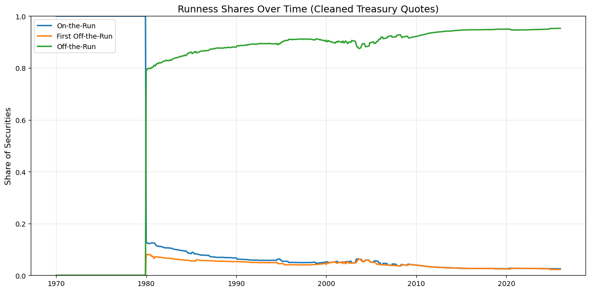
Above, we observe how before the early 1980s, all cleaned quotes are classified as “on-the-run.” This reflects limitations in historical issuance coverage & runnness identification in the early CRSP data. After 1980, the cross-section stabilizes, with ~80-95% of bonds off-the-run, and small shares of on-the-run and first-off-the-run securities.

5. Yield Curve Snapshot

To connect our cleaned dataset to the analysis code, we can build a quick yield curve snapshot figure via GSW’s implementation. This is not a full GSW curve estimation, but it illustrates why we want clean maturities, clean quotes, and runness labels for estimation.

# Choose a representative date (latest in sample)
snap_date = pd.to_datetime(df_tidy['date']).max()
snap = df_tidy.loc[pd.to_datetime(df_tidy['date']) == snap_date].copy()

# Basic "safe" screen for plotting
snap = snap.loc[
    snap['clean'] &
    (~snap['is_flower']) &
    (~snap['is_under_30d']) &
    (~snap['is_20yr_post_1996'])
]

print('snapshot date:', snap_date.date())
print('number of securities:', len(snap))

# Scatter: yield vs maturity (years)
fig, ax = plt.subplots(figsize=(9,4))
ax.scatter(snap['ttm_years'], snap['yield'], s=10, alpha=0.5, label='all (screened)')
ax.set_title('Snapshot: yield vs time-to-maturity', fontsize=14)
ax.set_xlabel('TTM (years)')
ax.set_ylabel('Yield')
plt.show()

snapshot date: 2026-01-30
number of securities: 368

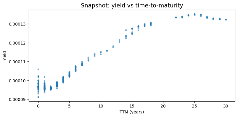
The first figure plots yield against time-to-maturity for all screened securities on the most recent date in the sample. Several features confirm the integrity of the cleaned dataset:

• The cross section spans the full maturity spectrum, confirming that the time-to-maturity calculation and maturity filtering steps in the pipeline are functioning as intended

• The curve has a smooth upward-sloping shape across most maturities, consistent with a typical positive term premium environment

• An absence of extreme outliers or discontinuities reflects the effectiveness of the cleaning flags

• Tight clustering of points at key maturity buckets reflects Treasury issuance conventions

#on-the-run vs off-the-run on same snapshot
fig, ax = plt.subplots(figsize=(9,4))
on = snap.loc[snap['is_on_the_run']]
off = snap.loc[snap['is_off_the_run']]
ax.scatter(on['ttm_years'], on['yield'], s=20, alpha=0.5, label='on-the-run')
ax.scatter(off['ttm_years'], off['yield'], s=10, alpha=0.35, label='off-the-run')
ax.set_title('Snapshot: yield vs time-to-maturity', fontsize=14)
ax.set_xlabel('TTM (years)')
ax.set_ylabel('Yield')
ax.legend()
plt.show()

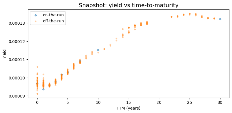
The second figure separates on-the-run and off-the-run securities within the same snapshot and highlights one of our motivations for constructing runness classifications in the cleaning pipeline. On-the-run securities are fewer in number and typically cluster at standard benchmark maturities. Off-the-run securities are much more numerous and fill in the maturity spectrum between benchmarks. In many maturity buckets, off-the-run securities exhibit slightly higher yields relative to nearby on-the-run bonds. This cross-sectional dispersion is exactly why runnness indicators are valuable inputs for term structure analysis.

6. The Output & How It Is Used

The pipeline writes the tidy_CRSP_treasury.parquet file. This tidy dataset is intended to be the single cleaned input for later steps, including:

• filtering to a curve-estimation sample (e.g., exclude bills / flower bonds / ultra-short maturities)

• estimating curve performance via Weighted Mean Absolute Errors (WMAE) & Hit Rates

• analyze differences between on-the-run and off-the-run securities

In other words, this tidy dataset serves as the foundation for all downstream term structure analysis. By consolidating cleaning and feature engineering into a single pipeline, later code can focus on estimation and evaluation rather than repeated data preparation.

7. Downstream Analysis Example: Fit Error Metrics

To connect this notebook to the replication code, we can inspect model fit metrics generated by:

• run_mcc_yield_curve.py

• run_fisher_yield_curve.py

• run_waggoner_yield_curve.py

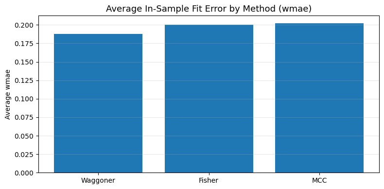
These scripts write error summaries into _data (for example mcc_error_metrics.csv). Below we load whichever files are available and compare average in-sample error across methods.

metrics_files = {
    'MCC': DATA_DIR / 'mcc_error_metrics.csv',
    'Fisher': DATA_DIR / 'fisher_error_metrics.csv',
    'Waggoner': DATA_DIR / 'waggoner_error_metrics.csv',
}

frames = []
for method, path in metrics_files.items():
    if path.exists():
        tmp = pd.read_csv(path)
        tmp['method'] = method
        frames.append(tmp)

if frames:
    metrics = pd.concat(frames, ignore_index=True)
    display(metrics.head())

    numeric_cols = metrics.select_dtypes(include=[np.number]).columns.tolist()
    preferred = [c for c in ['wmae', 'mae', 'rmse'] if c in numeric_cols]
    score_col = preferred[0] if preferred else (numeric_cols[0] if numeric_cols else None)

    if score_col is not None:
        summary = (
            metrics.groupby('method', as_index=False)[score_col]
            .mean()
            .sort_values(score_col)
            .rename(columns={score_col: f'avg_{score_col}'})
        )
        display(summary)

        fig, ax = plt.subplots(figsize=(8, 4))
        ax.bar(summary['method'], summary[f'avg_{score_col}'])
        ax.set_title(f'Average In-Sample Fit Error by Method ({score_col})', fontsize=13)
        ax.set_ylabel(f'Average {score_col}')
        ax.grid(axis='y', alpha=0.3)
        plt.tight_layout()
        plt.show()
    else:
        print('Error-metric files found, but no numeric score column was detected.')
else:
    print(
        'No error metric files found yet. Run curve tasks first, e.g. '
        '`doit build_mcc_yield_curve build_fisher_yield_curve build_waggoner_yield_curve`.'
    )

	bucket	wmae	hit_rate	method
0	0-1	0.027273	0.340641	MCC
1	1-3	0.106646	0.450051	MCC
2	3-5	0.271146	0.273383	MCC
3	5-10	0.421262	0.200919	MCC
4	>10	0.322544	0.288101	MCC

	method	avg_wmae
2	Waggoner	0.187894
0	Fisher	0.200445
1	MCC	0.202326